Getting Started
Installation
A key feaure of PottsPlayground is support for GPU acceleration, however PottsPlayground can compile and run without GPU support as well. For now, PottsPlayground is available as a source install via pip install PottsPlayground. If the setup process finds nvcc (the compiler for Nvidia GPU support) PottsPlayground will attempt to build for GPU execution; otherwise, it will build for CPU only. Note that even if nvcc is installed, it might not be on the system path. PottsPlayground prints a GPU status report when imported, which will indicate if it was built with or without GPU support, and whether or not the module can find a GPU to use.
Using Built-in Tasks
A few example tasks are built-in as a reference and for easy benchmarking. To create a random instance of the traveling salesman problem and “solve” for it’s minimum tour length, all one needs to do is:
import PottsPlayground

PottsTask = PottsPlayground.Tasks.TravelingSalesman(ncities=10, ConstraintFactor=1.5)

temp = PottsPlayground.Schedules.SawtoothTempLog2Space(MaxTemp=1., MinTemp=0.05, nTeeth=3, nIters=1e4)

results = PottsPlayground.Anneal(PottsTask, temp)

final_best_soln = results['MinStates'][-1,:]

PottsTask.DisplayState(final_best_soln)
Which should yield a plot of a tour somewhat like this:
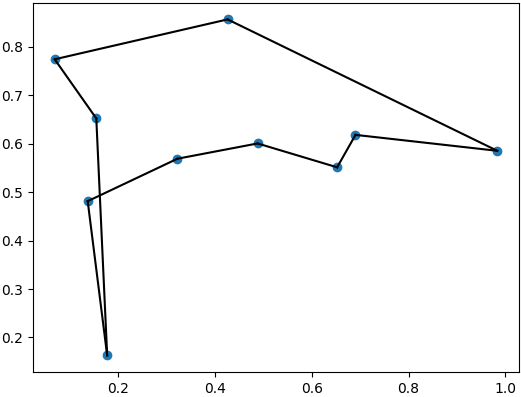
Which is obviously not an optimal solution, but increasing the number of iterations, details of the annealing algorithm, etc. can get you there.
Creating a New Task
New/custom tasks can be created using the BaseTask class, which is what the built-in examples do internally. For example, PottsPlayground can be used to create a 3-spin Ising model of an AND gate like so:
#manually create an Ising model of a logical AND gate, C = A&B

import numpy
import PottsPlayground
from PottsPlayground.Kernels import BinaryQuadratic as BQK

andgate = PottsPlayground.PottsModel()

#three variables, each which take on values of 0 or 1
andgate.AddSpins([2,2,2], ['A', 'B', 'C'])

#BQK is the binary quadratic kernel,
#which allows the simplification of the Potts Hamiltonian to the Ising Hamiltonian:
#Potts: E = sum Wij(mi,mj) ->
#Binary Quadratic Ising: E = sum Wij*mi*mj with m valued as 0 or 1
andgate.AddWeight(BQK, 'A', 'B', weight=1)
andgate.AddWeight(BQK, 'A', 'C', weight=-2)
andgate.AddWeight(BQK, 'B', 'C', weight=-2)

andgate.AddBias('C', [0,3]) #other two Spins need no biases

andgate.Compile()

#run the model at a constant temperature to capture statistics:
temp = PottsPlayground.Schedules.constTemp(niters=1e6, temp=1)
results = PottsPlayground.Anneal(andgate, temp, nReports=int(1e4))

samples = results["AllStates"]
sample_indices = (samples[:,0, andgate.IndexOf('A')]
                                +2*samples[:,0,andgate.IndexOf('B')]
                                +4*samples[:,0,andgate.IndexOf('C')])
unique, counts = numpy.unique(sample_indices, return_counts=True)

for i, c in zip(unique, counts):
        pr = c/sample_indices.shape[0]
        print("Pr(A=%i, B=%i, C=%i) = %.3f"%(i%2, (i/2)%2, (i/4)%2, pr))
Which when run should yield a set of probabilities where the valid states where C = A & B is true are all equally likely, and the invalid states are unlikely:
C = A & B
Pr(A=0, B=0, C=0) = 0.194
Pr(A=1, B=0, C=0) = 0.195
Pr(A=0, B=1, C=0) = 0.191
Pr(A=1, B=1, C=0) = 0.075
Pr(A=0, B=0, C=1) = 0.007
Pr(A=1, B=0, C=1) = 0.069
Pr(A=0, B=1, C=1) = 0.071
Pr(A=1, B=1, C=1) = 0.199
In general, sucessfully representing more complicated tasks as Potts models benefits from more structured code for calculating weights and tabulating the mapping between Potts spins and task semantics.